[Haptics - Dynamic compensation] Calibration Using NI DAQ, Python and Matlab

이번 게시글에서는 앞서 포스팅한 게시글

https://sillon-coding.tistory.com/631

[Haptics - Dynamic compensation] Matlab에서 Chirp Signal 출력하기

 

에서 추출한 Chirp Signal을 바탕으로 30~ 300 Hz 주파수 대역에서 진동을 사용하도록 Calibaration 을 진행할것입니다.

 

간단히 코드만 짚고 넘어가겠습니다.

chirp_test.m (matlab 코드입니다.) 

% 샘플링 레이트 및 시간 벡터 설정
Fs = 10000;  % 샘플링 주파수 (Hz)
T = 10;       % 총 지속 시간 (초)
t = linspace(0, T, Fs * T); % 시간 벡터

% Chirp Signal 생성 (30Hz -> 300Hz)
f0 = 30;  % 시작 주파수 (Hz)
f1 = 300; % 종료 주파수 (Hz)
y = chirp(t, f0, T, f1);

% 생성된 신호 플로팅
figure;
plot(t, y);
xlabel('Time (s)');
ylabel('Amplitude');
title('Chirp Signal (30Hz to 300Hz)');
grid on;

% 텍스트 파일로 저장
fileID = fopen('chirp_signal.txt', 'w');
fprintf(fileID, '%f\n', y);
fclose(fileID);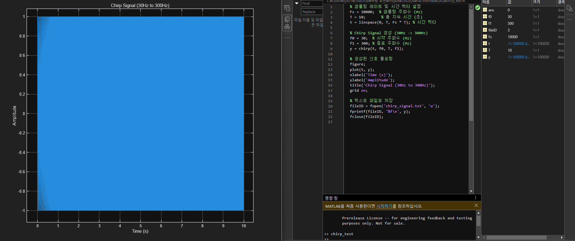

 

In [10]:

# Modules

import nidaqmx
import nidaqmx.system
import numpy as np
import datetime

 

 

Acceleration Using Chirp Signal¶

 

In [11]:

## Variable Definition
samplingRate = 10000
duration = 10
ReadCh = 3
now = datetime.datetime.now()

 

In [12]:

import csv
import os

def DFT321(Arr):
    DFTArr = []

    U_temp = np.zeros((samplingRate * duration, 3)) * 1j
    U_temp[:,0] = np.fft.fft(Arr[0])
    U_temp[:,1] = np.fft.fft(Arr[1])
    U_temp[:,2] = np.fft.fft(Arr[2])
    Y_temp = np.zeros((samplingRate * duration//2 + 1, 1)) * 1j

    for i in range(samplingRate * duration//2 + 1):
        absY = np.real(np.sqrt(np.pow(abs(U_temp[i][0]), 2) + np.pow(abs(U_temp[i][1]), 2) + np.pow(abs(U_temp[i][2]), 2)))
        PhaseChoice = np.angle(sum(U_temp[i]))
        Y_temp[i] = absY * np.exp(1j * PhaseChoice)

    Y_flip = np.conj(np.flip(Y_temp))
    Y = np.concat((Y_temp, Y_flip[2:]))
    DFTArr = abs(np.real(np.fft.ifft(Y)))

    return DFTArr

def saveData(Arr, Date, T_start):
    dir = os.getcwd()
    SaveArr = np.zeros((1 + ReadCh + 1 + 1 + 1, samplingRate * duration))
    for i in range(samplingRate * duration):
        SaveArr[0][i] = T_start + 0.1 * i
        SaveArr[1][i] = Arr[0][i]
        SaveArr[2][i] = Arr[1][i]
        SaveArr[3][i] = Arr[2][i]
        # SaveArr[4][i] = # DFT
        # SaveArr[5][i] = # Speed
        if i == 0:
            SaveArr[5][i] = 0
        else:
            SaveArr[5][i] = (SaveArr[4][i] - SaveArr[4][i-1]) * samplingRate
            
    SaveArr[4] = DFT321(Arr).squeeze()
    print(np.shape(DFT321(Arr)))



    f = open("Accel//Accels_" + Date + ".txt", 'a')
    for i in range(samplingRate * duration):
        line = str(SaveArr[0][i]) + ", " + str(SaveArr[1][i]) + ", " + str(SaveArr[2][i]) + ", " + str(SaveArr[3][i]) + ", " + str(SaveArr[4][i]) + ", " + str(SaveArr[5][i]) + ", " + str(SaveArr[6][i]) + "\n"
        f.write(line)
    f.close()

 

In [13]:

## DAQ Ready
system = nidaqmx.system.System.local()
for device in system.devices:
    print(device)
device = system.devices['Dev1']
# out_chan = device.ao_physical_chans['ao0']
in_chan = device.ai_physical_chans['ai0:2']

 

 

Device(name=Dev1)

 

 

Matlab에서 생성한 Chrip Signal 불러오기¶

 

In [14]:

# 파일 경로 지정
file_path = "chirp_signal.txt"

with open(file_path, 'r') as file:
    lines = file.readlines()
    signal_data = [float(line.strip()) for line in lines if line.strip()]
signal_data 

 

Out[14]:

[1.0,
...
 0.676431,
 ...]

 

In [17]:

import time

for i in range(10):

    readtask = nidaqmx.Task()
    writetask = nidaqmx.Task()

    readtask.ai_channels.add_ai_voltage_chan("Dev1/ai0:2", terminal_config=nidaqmx.constants.TerminalConfiguration.RSE, min_val=-10, max_val=10)
    readtask.timing.cfg_samp_clk_timing(samplingRate, sample_mode=nidaqmx.constants.AcquisitionType.FINITE, samps_per_chan=samplingRate * duration)
    writetask.ao_channels.add_ao_voltage_chan("Dev1/ao0")
    writetask.timing.cfg_samp_clk_timing(samplingRate, sample_mode=nidaqmx.constants.AcquisitionType.FINITE, samps_per_chan=samplingRate * duration)

    writetask.write(signal_data)
    writetask.start()

    data = readtask.read(samplingRate * duration)

    writetask.wait_until_done()
    writetask.close()
    readtask.close()


    f = open("./Chirp/Chirp_Accels_"+str(i)+".txt" , "a")
    for j in range(samplingRate * duration):
        f.write(f"{data[0][j]}\n")
    f.close()


    time.sleep(2)

 

In [19]:

# 마지막으로 측정한 데이터의 파형 보기기
plt.plot(data[0]) # X
plt.show()
plt.plot(data[1]) # Y
plt.show()
plt.plot(data[2]) # Z
plt.show()

 

 

 

 

 

In [35]:

import numpy as np
def Mean_accels_data(title):
    num_measurements = 10  # 반복 횟수
    target_length = 100000

    all_measurements = []

    for i in range(num_measurements):
        data = np.loadtxt(f"{title}_{i}.txt", delimiter=",")  # 데이터 파일 불러오기
        
        # 데이터 길이 조정 (Zero Padding 또는 Truncation)
        if len(data) > target_length:
            data = data[:target_length]  # 길이가 길 경우 자름
        # else:
        #     padded_data = np.pad(data, (0, target_length - len(data)), 'constant', constant_values=0)
        
        all_measurements.append(data)

    # NumPy 배열 변환 후 평균 계산
    all_measurements = np.array(all_measurements)
    average_data = np.mean(all_measurements, axis=0)

    plt.figure(figsize=(10, 5))
    plt.plot(average_data, label="Mean Acceleration")
    plt.xlabel("Samples")
    plt.ylabel("Acceleration")
    plt.legend()
    plt.grid()
    plt.show()

    return average_data

 

 

Chirp Signal Mean plot¶

 

In [36]:

average_data = Mean_accels_data('Chirp/Chirp_Accels')

 

 

 

 

save mean data

 

In [38]:

print(average_data)

f = open("Chirp/Chirp_Accels_Mean.txt" , "a")
for j in range(len(average_data)):
    f.write(f"{average_data[j]}\n")
f.close()

 

 

[0.97474134 0.97271213 0.97152037 ... 0.92459089 0.92420437 0.92484857]

 

In [ ]:

 

이제 여기서 Chirp Signal의 평균을 보정해주는 식을 찾겠습니다.

dynamic_compensation.m

 

%% 전역변수
samplingRate = 10000;
time = 10;
samps = samplingRate * time;
fmin = 30;
fmax = 300;
voltage = 1;
t = linspace(0, time, samps);
f = linspace(0, samplingRate, samps);
iodelay = 0;
Ts = 1/samplingRate;
PI = 3.1415926536;



%% 입력
chrpName=sprintf('chirp_signal.txt');
fileName=sprintf('Chirp\\Chirp_Accels_Mean.txt');
chrp = textread(chrpName, '%f');
mtr = textread(fileName, '%f');
tr = mtr - mean(mtr);
HighpassedMotor = highpass(tr, fmin, samplingRate, 'Steepness', 0.9);

chrp = chirp(t, fmin, 1, fmax);
%%
fftChirp = fft(chrp);
fftOutput = fft(HighpassedMotor);
%InversetransferFunction = fftChirp ./ fftOutput;

%input output data encapsulation
%iddataTF = iddata(HighpassedMotor, chrp, 1/samplingRate);
iddataITF = iddata(chrp', HighpassedMotor, 1/samplingRate);

EstimatedITF = etfe(iddataITF, [], samplingRate*time);
%etfe Smoothing

[TFmag, TFphase, TFwout] = bode(EstimatedITF);
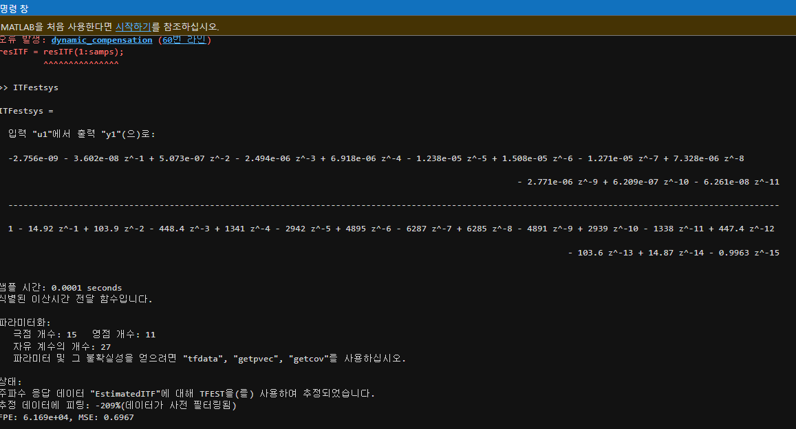
TFestsys = tfest(EstimatedITF, 14,12 , iodelay, 'Ts', Ts, 'Feedthrough', true, tfestOptions('WeightingFilter', [30*(2*PI), 300*(2*PI)]));

compare(ITFestsys, EstimatedITF);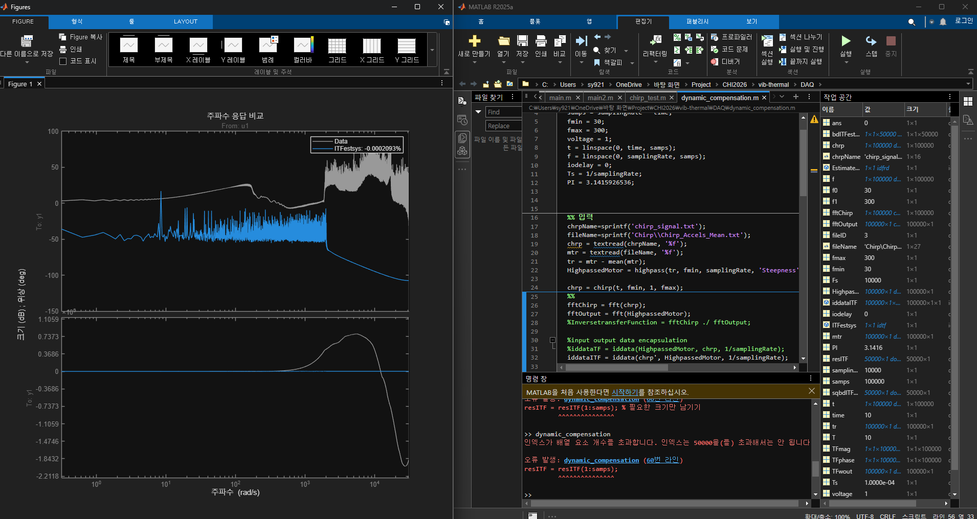

현재 그래프(이미지)와 조정해야 할 부분 연결하기

현재 MATLAB의 compare(ITFestsys, EstimatedITF);에서 나타난 파란색(측정된 ITF)과 회색(추정된 ITF) 그래프가 겹쳐져야 한다.
즉, 추정된 전달 함수(Identified Transfer Function, ITF)가 실제 측정된 데이터와 일치하도록 조정해야 한다.

---

1️⃣ 그래프 분석 (회색 vs. 파란색)

• 회색 그래프: 현재 모델이 추정한 주파수 응답(Estimated ITF)
• 파란색 그래프: 실제 측정된 가속도 응답(실제 ITF 데이터)
• 차이점: 일부 주파수 구간에서 두 그래프가 일치하지 않고 차이가 발생함

📌 이 차이를 줄이려면, 전달 함수의 차수(14,12)를 조정해야 한다.
차수가 너무 낮으면 전체적인 경향을 따라가지 못하고, 너무 높으면 특정 구간에서만 잘 맞을 수 있으므로,
최적의 차수를 찾아야 한다.

---

2️⃣ 해결 방법: tfest() 함수의 전달 함수 차수 조정

MATLAB의 tfest()를 사용하여 전달 함수(Transfer Function)의 차수를 조정할 수 있다.

ITFestsys = tfest(EstimatedITF, 14, 12, iodelay, 'Ts', Ts, ... 'Feedthrough', true, tfestOptions('WeightingFilter', [30*(2*PI), 300*(2*PI)]));

• 14,12: 현재 사용된 전달 함수의 차수 (분자 14차, 분모 12차).
• iodelay: 입출력 지연값.
• 'WeightingFilter': 특정 주파수 대역(30Hz~300Hz)에서 성능을 최적화하도록 설정.

차수를 조정하는 이유

• 전달 함수의 차수가 너무 낮으면, 모델이 단순해져서 전체적인 주파수 응답을 충분히 따라가지 못한다.
• 전달 함수의 차수를 조정하면, 모델이 실제 측정값(파란색)과 더 유사한 주파수 응답을 보이도록 개선할 수 있다.
• 적절한 차수를 찾으면 전 주파수 대역에서 파란색과 회색이 최대한 일치하도록 조정할 수 있다.

---

3️⃣ 차수 변경에 따른 조정

차수를 조정하면서 파란색과 회색이 더 잘 겹치는 값을 찾을 수 있다.
예를 들어:

ITFestsys = tfest(EstimatedITF, 18, 16, iodelay, 'Ts', Ts, ... 'Feedthrough', true, tfestOptions('WeightingFilter', [30*(2*PI), 300*(2*PI)]));

또는

ITFestsys = tfest(EstimatedITF, 20, 18, iodelay, 'Ts', Ts, ... 'Feedthrough', true, tfestOptions('WeightingFilter', [30*(2*PI), 300*(2*PI)]));

이렇게 차수를 높이거나 낮추면서 파란색과 회색이 최대한 겹치는 값을 찾으면 된다. 

---

4️⃣ 결론

• 현재 compare(ITFestsys, EstimatedITF);의 결과에서 회색(추정값)과 파란색(실제 측정값)이 일치하도록 조정해야 한다.
• 이를 위해 tfest()의 전달 함수 차수(14,12)를 바꿔가면서 실험해야 한다.
• 차수가 너무 낮으면 전체적인 경향을 따라가지 못하고, 너무 높으면 특정 구간에서만 잘 맞을 수 있으므로 최적의 차수를 찾는 것이 중요하다.
• 차수를 높이면 세밀한 주파수 응답을 추정할 수 있으며, 이를 통해 모델이 실제 데이터를 최대한 반영하도록 조정할 수 있다.

📌 최종 목표: 파란색과 회색이 최대한 겹치는지 확인하면서 전달 함수 차수를 조정하여, 측정된 데이터를 최대한 반영한 모델을 만드는 것이다.

 

ITFestsys = tfest(EstimatedITF, 15,11 , iodelay, 'Ts', Ts, 'Feedthrough', true, tfestOptions('WeightingFilter', [30*(2*PI), 300*(2*PI)]));

 

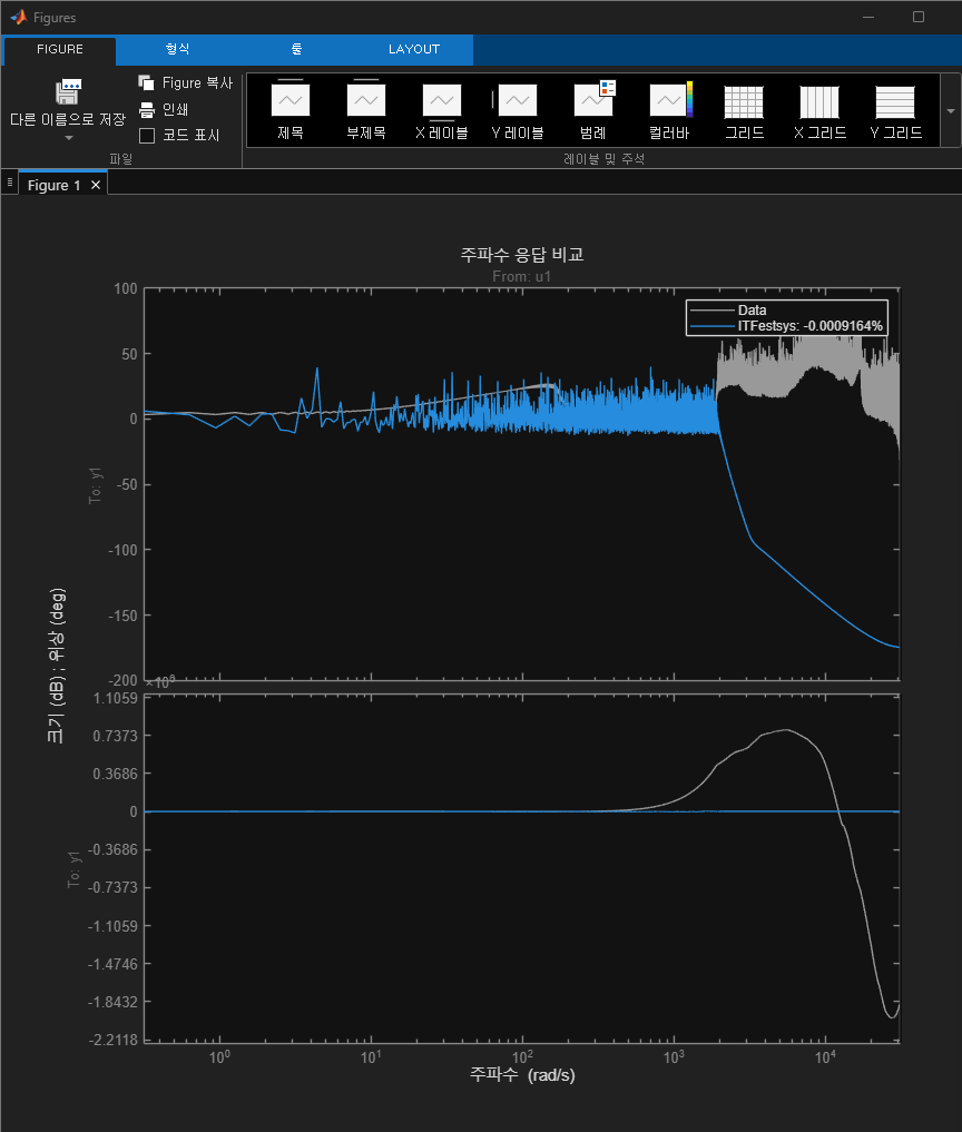
차수를 높게 한다고 잘되는건 아니다. (되도록 9 안의 값을 찾으면서 찾자)

 

차수 예시는 아래와 같음